Numerical Algorithms using Playgrounds

There’s nothing like lines on graph paper to bring back nightmares from high school.

Hopefully you didn’t vomit when read numerical algorithms. If you did, well, look on the bright side … you can have lunch again! :]

In this tutorial, you’ll learn what numerical algorithms are and how to use them to solve problems that don’t have an analytic solution. You’ll also learn how you can use playgrounds to easily visualize the solutions.

If the notion of math doesn’t excite you, nor are you an avid user of physics or computer science, you’ll still find value in this tutorial. All you need is a basic understanding of calculus and some elementary physics.

You’ll learn how to solve two different problems with numerical algorithms, but for the sake of learning, both also allow analytic solutions. Though algorithms are ideal for those times when analytics won’t work, it’s easier to understand how they work when you can compare the two methodologies.

What are Numerical Algorithms?

Simply put, numerical algorithms are methods to solve mathematical problems that don’t rely on a closed-form analytic solution.

What is a Closed-Form Analytic Solution?

It’s any mathematical formula that you use to solve an exact value by plugging in the values you already know and performing a finite set of operations.

More simply put, if you can use algebra to find an expression to solve an unknown value, and all you need to do is substitute the known values and evaluate that expression, then you have a closed-form analytic solution.

When to Use Numerical Algorithms

For many problems, no analytic solution exists. For others, there is, but it would take too long to calculate, and In these cases, you need numerical algorithms. 

For example, imagine that you wrote a physics engine that computes the behavior of many objects in a limited amount of time. In this scenario, you can use numerical algorithms to calculate the behavior much faster.

There is a downside: You pay for the faster calculation with less precise results. But in many cases, the result is good enough.

Weather forecasting is example of an activity that benefits from the use of numerics. Think about how quickly it evolves and how many factors affect it; it’s a highly complex system and only numerical simulations can handle the task of predicting the future.

Maybe a lack of these algorithms is why your iPhone tells you that it’s raining but a look outside says the opposite!

Getting Started

As a warm up, you’ll play a game, and then you’ll calculate the square root of a given number. For both tasks, you’ll use the bisection method. Surprise! You probably know this method, but maybe not by name.

Think back to the childhood game where you choose a number between one and 100, and then someone else has to guess it. The only hint you can give the other person is if the number is bigger or smaller than the guess.

Let’s say you’re guessing what I’ve chosen, and you start with one. I tell you the number is higher. Then you choose two, and again, I tell you it’s higher. Now you choose three, then four, and each time I tell you the number is bigger, until you get to five, which is my number.

After five steps you find the number — not bad — but if I chose 78, this approach would take quite a bit of time.

This game moves much faster when you use the bisection method to find the solution.

The Bisection Method

You know the number is inside the interval [1,100], so instead of making incremental or even random guesses, you divide this interval into two subintervals of the same size: a=[1,50] and b=[51,100].

Then you determine if the number is inside interval a or b by asking if the number is 50. If the number is smaller than 50, you forget interval b and subdivide interval a again.

Then you repeat these steps until you find the number. Here’s an example:

My number is 60, and the intervals are a=[1,50] and b=[51,100].

In the first step, you say 50 to test the upper bound of interval a. I tell you the number is bigger, and now you know that the number is in interval b. Now you subdivide b into the intervals c=[51,75] and d=[76,100]. Again, you take the upper bound of interval c, 75, and my answer is that the number is smaller. This means the number must be in interval c, so you subdivide again

By using this method, you find the number after just seven steps versus 60 steps with the first approach.

1. 50 -> bigger
2. 75 -> smaller
3. 62 -> smaller
4. 56 -> bigger
5. 59 -> bigger
6. 61 -> smaller
7. 60 -> got it

For the square root of a number x, the process looks similar. The square root is between 0 and x, or expressed as an interval it is (0, x]. If the number is bigger than or equal to 1. You can use the interval [1, x].

Dividing this interval brings you to a=(0, x/2] and b=(x/2, x].

If my number is 9, the interval is [1, 9] the divided intervals are a=[1, 5] and b=(5, 9]. The middle m is (1+9)/2 = 5.

Next, you check if m*m – x is bigger than the desired accuracy. Is this case, you check if m*m is bigger or smaller than x. If it’s bigger, you use the interval (0,x/2] otherwise (x/2,x]

Let’s see this in action, we start with m=5 and a desired accuracy of 0.1:

1. Calculate m*m-x: 5*5-9 = 16
2. Check if the desired accuracy is reached: 25-11 <= 0.1 ?
3. Search next interval: Is m*m greater than x? Yes 25 is greater than 9, now use the interval [1, 5] with a middle of (1+5)/2 = 3
4. Calculate m*m-x: 3*3-9 = 0
5. Check if the desired accuracy is reached: 9-9 <= 0.1 ?
6. Got it.

Taking Bisection to Playgrounds

At this point, you’re going to take the theory and put it into practice by creating your own bisection algorithm. Create a new playground and add the following function to it.

func bisection(x: Double) -> Double {
//1
    var lower = 1.0
    //2
    var upper = x
    //3
    var m = (lower + upper) / 2
    var epsilon = 1e-10
    //4
    while (fabs(m * m - x) > epsilon) {
    //5
        m = (lower + upper) / 2
        if m * m > x {
            upper = m
        } else {
            lower = m
        }
    }

    return m
}

What does each section do?

1. Sets the lower bound to 1
2. Sets the upper bound to x
3. Finds the middle and defines the desired accuracy
4. Checks if the operation has reached the desired accuracy
5. If not, this block finds the middle of the new interval and checks which interval to use next

To test this function, add this line to your playground.

let bis = bisection(2.5)

As you can see on the right of the line m = (lower + upper) / 2, this code executes 35 times, meaning this method takes 35 steps to find the result.

Now you’re going to take advantage of one of the loveable features of playgrounds — the ability to view the history of a value.

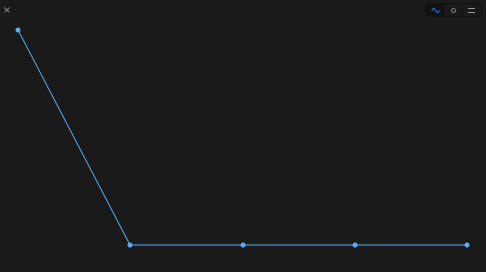
Since the bisection algorithm successively calculates more accurate approximations of the actual solution, you can use the value history graph to see how this numerical algorithm converges on the correct solution.

Press option+cmd+enter to open the assistant editor, and then click on the rounded button on the right side of the line m = (lower + upper) / 2 to add a value history to the assistant editor.

Here you can see the method jumping around the correct value.

Ancient Math Still Works

The next algorithm you’ll learn dates back to antiquity. It originated in Babylonia, as far back as 1750 B.C, but was described in Heron of Alexandria’s book Metrica around the year 100. And this is how it came to be known as Heron’s method. You can learn more about Heron’s method over here.

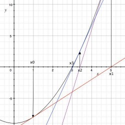
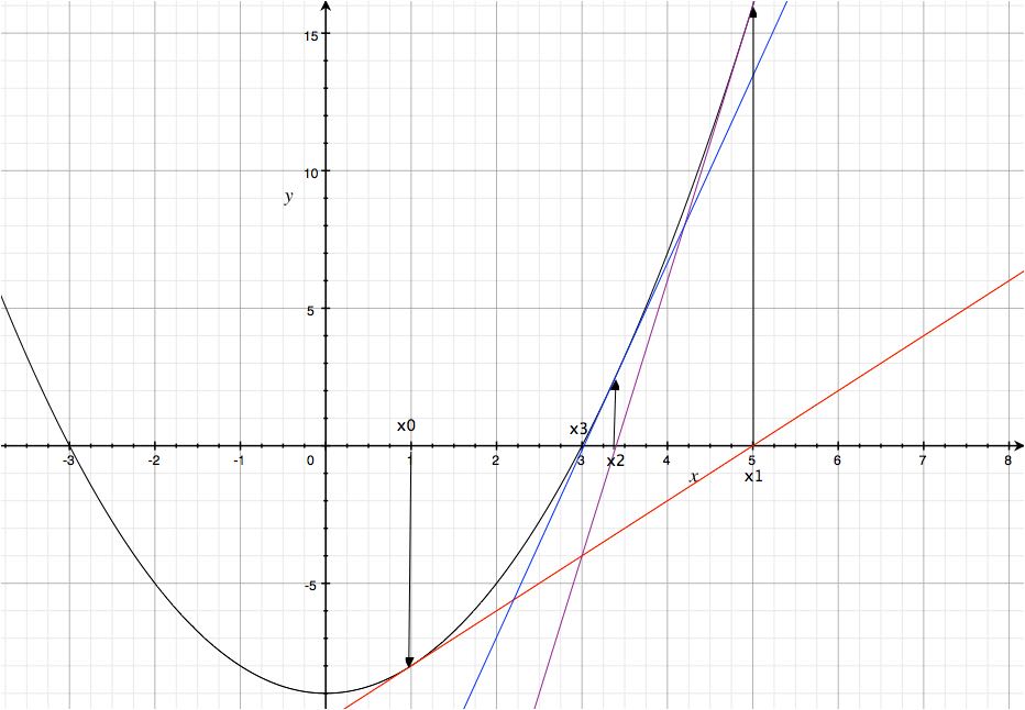
This method works by using the function , where a is the number for which you want to calculate the square root. If you can find this curve’s zero point — the value of x where the function equals zero — then you have found the square root of a.

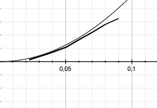
To do this, you start with an arbitrary starting value of x, calculate the tangent line at this value, and then find the tangent line’s zero point. Then you repeat this using that zero point as the next starting value, and keep repeating until you reach the desired accuracy.

Since every tangent moves closer to true zero, the process converges on the true answer. The next graphic illustrates this process by solving with a=9, using a starting value of 1.

The starting point at x0=1 generates the red tangent line, producing the next point x1 that generates the purple line, producing the x2 that generates the blue line, finally leading to the answer.

Ancient Math, Meet Playgrounds

You have something that the Babylonians did not: playgrounds. Check out what happens when you add the following function to your playground:

func heron(x: Double) -> Double {
  //1
  var xOld = 0.0
  var xNew = (x + 1.0) / 2.0
  var epsilon = 1e-10

  //2
  while (fabs(xNew - xOld) > epsilon) {
    //3
    xOld = xNew
    xNew = (xOld + x / xOld) / 2
  }

  return xNew
}

What’s happening here?

1. Creates variables to store the current result. xOld is the last calculated value andxNew the actual value.
   • A good starting point for this method is found the way xNew is initialized.
   • epsilon is the desired accuracy.
   • In this case, you calculate the square root up to the 10th decimal place.
2. While checks if the desired accuracy is reached.
3. If not, xNew becomes the new xOld, and then the next iteration starts.

Check your code by adding the line:

let her = heron(2.5)

Heron method requires only five iterations to find the result.

Click on the rounded button on the right side of the line xNew = (xOld + x / xOld) / 2 to add a value history to the assistant editor, and you’ll see that the first iteration found a good approximation.

Meet Harmonic Oscillators

In this section, you’ll learn how to use numerical integration algorithms in order to model a simple harmonic oscillator, a basic dynamical system.

The system can describe many phenomena, from the swinging of a pendulum to the vibrations of a weight on a spring, to name a couple. Specifically, it can be used to describe scenarios that involve a certain offset or displacement that changes over time.

You’ll use the playground’s value history feature to model how this offset value changes over time, but won’t use it to show how your numerical approximation takes you successively closer to the perfect solution.

For this example, you’ll work with a mass attached to a spring. To make things easier, you’ll ignore damping and gravity, so the only force acting on the mass is the spring force that tries to pull the mass back to an offset position of zero.

With this assumption, you only need to work with two physical laws.

• Newton’s Second Law: , which describes how the force on the mass changes its acceleration.
• Hook’s Law:, which describes how the spring applies a force on the mass proportional to its displacement, where k is the spring constant and x is the displacement.

Harmonic Oscillator Formula

Since the spring is the only source of force on the mass, you combine these equations and write the following:

You can write this as:

is also known as , which is the square of the resonance frequency.

The formula for the exact solution is as follows:

A is the amplitude, and in this case it means the displacement, , is known as phase difference. Both are constant values that can be found using initial values.

If you say at the time t=0 you have and you find the amplitude and phase difference as:

Let’s look at an example. We have a mass of 2kg attached to a spring with a spring constant k=196N/m. At the time t=0 the spring has a displacement of 0.1m. To calculate and we have to calculate .

and

Take it to the Playground

Before you use this formula to calculate the exact solution for any given time step, you need to write some code.

Go back to your playground and add the following code at the end:

//1
typealias Solver = (Double, Double, Double, Double, Double) -> Void

//2
struct HarmonicOscillator {
  var kSpring = 0.0
  var mass = 0.0
  var phase = 0.0
  var amplitude = 0.0
  var deltaT = 0.0

  init(kSpring: Double, mass: Double, phase: Double, amplitude: Double, deltaT: Double) {
    self.kSpring = kSpring
    self.mass = mass
    self.phase = phase
    self.amplitude = amplitude
    self.deltaT = deltaT
  }

  //3
  func solveUsingSolver(solver: Solver) {
    solver(kSpring, mass, phase, amplitude, deltaT)
  }
}

What’s happening in this block?

1. This defines a typealias for a function that takes five Double arguments and returns nothing.
2. Here you create a struct that describes a harmonic oscillator.
3. This function simply creates Closures to solve the oscillator.

Compare to an Exact Solution

The code for the exact solution is as follows:

func solveExact(amplitude: Double, phase: Double, kSpring: Double, mass: Double, t: Double) {
  var x = 0.0
  //1
  let omega = sqrt(kSpring / mass)

  var i = 0.0

  while i < 100.0 {
//2
    x =  amplitude * sin(omega * i + phase)
    i += t
  }
}

This method includes all the parameters needed to solve the movement equation.

1. Calculates the resonance frequency.
2. The current position calculates Inside the while loop, and i is incremented for the next step.

Test it by adding the following code:

let osci = HarmonicOscillator(kSpring: 0.5, mass: 10, phase: 10, amplitude: 50, deltaT: 0.1)
osci.solveUsingSolver(solveExact)

The solution function is a bit curious. It takes arguments, but it returns nothing and it prints nothing.

So what is it good for?

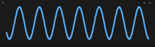
The purpose of this function is that, within its while loop, it models the actual dynamics of your oscillator. You'll observe those dynamics by using the value history feature of the playground.

Add a value history to the line x = amplitude * sin(omega * i + phase) and you'll see the oscillator moving.

Now that you have an exact solution working, you can start with the first numerical solution.

Euler Method

The Euler method is the simplest method for numerical integration. It was introduced in the year 1768 in the book Institutiones Calculi Integralis by Leonhard Euler. To learn more about the Euler method, you can find out here.

The idea behind this method is to approximate a curve by using short lines.

This is done by calculating the slope on a given point and drawing a short line with the same slope. At the end of this line, you calculate the slope again and draw another line. As you can see, the accuracy depends on the length of the lines.

Did you wonder what deltaT is used for?

The numerical algorithms you use have a step size, which is important for the accuracy of such algorithms; bigger step sizes cause lower accuracy but faster execution speed and vice versa.

deltaT is the step size for your algorithms. You initialized it with a value of 0.1, meaning that you calculated the position of the mass for every 0.1 second. In the case of the Euler method, this means that the lines have a length of 0.1 units on the x-Axis.

Before you start coding, you need to have a look again at the formula:

This second order differential equation can be replaced with two differential equations of first order.

can be written as and this as

You get this by using the difference quotient:

And you also get those:

With these equations, you can directly implement the Euler method.

Add the following code right behind solveExact:

func solveEuler(amplitude: Double, phase: Double, kSpring: Double, mass: Double, t: Double) {
  //1
  var x = amplitude * sin(phase)
  let omega = sqrt(kSpring / mass)
  var i = 0.0
  //2
  var v = amplitude * omega * cos(phase);
  var vold = v
  var xoldEuler = x

  while i < 100 {
    //3
    v -= omega * omega  * x * t
    //4
    x += vold * t
    xoldEuler = x

    vold = v
    i+=t
    }
}

What does this do?

1. Sets the current position and omega.
2. Calculates thee current speed.
3. Makes calculating the new velocity the first order of business inside the while loop.
4. The new position calculates at the end based on the velocity, and at the end, i is incremented by the step size t.

Now test this method by adding the following to the bottom of your playground:

osci.solveUsingSolver(solveEuler)

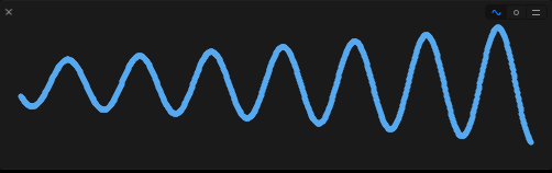
Then add a value history to the line xoldEuler = x. Take a look at the history, and you'll see that this method also draws a sine curve with a rising amplitude. The Euler method is not exact, and in this instance the big step size of 0.1 is contributing to the inaccuracy.

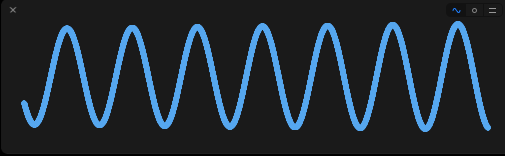
Here is another image, but this shows how it looks with a step size of 0.01, which leads to a much better solution. So, when you think about the Euler method, remember that it's most useful for small step sizes, but it also has the easiest implementation.

Velocity Verlet

The last method is called Velocity Verlet. It works off the same idea as Euler but calculates the new position a slightly different way.

Euler calculates the new position, while ignoring the actual acceleration, with the formula .

Velocity Verlet takes acceleration into account − this brings better results for the same step size.

Add the following code right after solveEuler:

func solveVerlet(amplitude: Double, phase: Double, kSpring: Double, mass: Double, t: Double) {
  //1
  var x = amplitude * sin(phase)
  var xoldVerlet = x
  let omega = sqrt(kSpring / mass)

  var v = amplitude * omega * cos(phase)
  var vold = v
  var i = 0.0

  while i < 100 {
    //2
    x = xoldVerlet + v * t + 0.5 * omega * omega * t * t
    v -= omega * omega * x * t
    xoldVerlet = x
    i+=t
  }
}

What's going on here?

1. Everything until the loop is the same as before.
2. Calculates the new position and velocity and increments i.

Again, test the function by adding this line to the end of your playground:

osci.solveUsingSolver(solveVerlet)

And also add a value history to the line xoldVerlet = x

Where to Go From Here?

You can download the completed project over here.

I hope you enjoyed your trip into the numerical world, learned a few things about algorithms, and even a few fun facts about the ancient world to help you on your next trivia night.

Before you start exploring more, you should play with different values for deltaT, but keep in mind that playgrounds are not that fast and choosing a small step size can freeze Xcode for a long time -- my MacBook froze for several minutes after I changed deltaT to 0.01 to make the second Euler screenshot.

With the algorithms you learned, you can solve a variety of problems like the n-body problem.

If you are feeling a little shaky about algorithms in general, you should check out MIT's Introductions to Algorithms class on YouTube.

Finally, keep check back to the site for more tutorials on this subject.

If you have questions or ideas about other ways to use numerical algorithms, bring it to the forums by commenting below. I look forward to hearing your thoughts and talking about all the cool things math can do for your apps.

The post Numerical Algorithms using Playgrounds appeared first on Ray Wenderlich.